Analytical benchmarks

Two analytical solutions from pytes.validation check the packed-bed model: Schumann’s solution for a bed of a sensible material, and the melting of a sphere (the spherical Stefan problem). Both models are built from the packed bed’s own submodels with pytes.ComposedModel (see composing models), swapping only what each benchmark needs.

import matplotlib.pyplot as plt
import numpy as np
import pybamm

import pytes
from pytes import validation
from pytes.materials import SensibleMaterial
from pytes.submodels import (
    BaseSubModel,
    DeviceEnergy,
    EnthalpyStorage,
    WallCoupling,
)
from pytes.submodels.storage import INITIAL_TEMPERATURE

base = pytes.PackedBedModel()
param = base.param
geometry = base.submodels["storage"].storage_geometry

Schumann: a sensible packed bed

The capsules are a sensible material, conductive enough to be lumped (Biot number 0.008), and the fluid enters at 70 °C into a bed at 32 °C. In Schumann’s variables, xi is the number of transfer units from the inlet and eta the time since the first fluid reached the outlet, in units of the particles’ time constant.

fluid = base.submodels["fluid"]
storage = EnthalpyStorage(param, SensibleMaterial("Capsule"), geometry, label="Capsule")
sensible = pytes.ComposedModel(
    {
        "fluid": fluid,
        "storage": storage,
        "coupling": WallCoupling(param, param.fluid, "Capsule", geometry),
        "device energy": DeviceEnergy(param, fluid, [storage]),
    },
    param,
    name="Sensible packed bed",
    defaults_from=base,
)
pv = base.default_parameter_values
pv.update(
    {
        "Capsule conductivity [W.m-1.K-1]": 1e3,
        "Capsule density [kg.m-3]": 1000,
        "Capsule specific heat capacity [J.kg-1.K-1]": 2000,
        "Heat transfer coefficient [W.m-2.K-1]": 300,
    },
    check_already_exists=False,
)
h, R, eps = 300, pv["Capsule radius [m]"], pv["Bed porosity"]
Z, A = pv["Bed length [m]"], pv["Bed cross-sectional area [m2]"]
rho_f = pv["Heat transfer fluid density [kg.m-3]"]
c_f = pv["Heat transfer fluid specific heat capacity [J.kg-1.K-1]"]
a = 3 * (1 - eps) / R
u = pv["Mass flow rate [kg.s-1]"] / (rho_f * eps * A)
xi = h * a * Z / (eps * rho_f * c_f * u)
rate = h * a / ((1 - eps) * 1000 * 2000)

t = np.linspace(0, 3000, 151)
exact = [validation.schumann(xi, rate * (ti - Z / u))[0] for ti in t]
fig, ax = plt.subplots(figsize=(6, 4))
for n_z in (50, 200, 400):
    solution = pybamm.Simulation(
        sensible, parameter_values=pv, var_pts={base.r: 5, base.z: n_z}
    ).solve([0, t[-1]], t_interp=t)
    theta = (solution["Outlet temperature [K]"].entries - 305.15) / 38
    ax.plot(t / 60, theta, label=f"{n_z} cells")
ax.plot(t / 60, exact, "k--", label="Schumann")
ax.set_xlabel("Time [min]")
ax.set_ylabel("Scaled outlet temperature")
ax.legend()
plt.show()

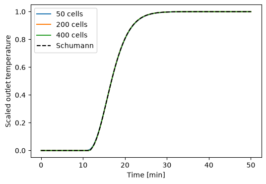
With the default, second-order scheme the model is within 1 % of Schumann’s solution on 50 cells. On finer meshes about 0.3 % is left: the difference between a capsule that conducts heat and Schumann’s lumped one. (With first-order upwinding, numerical diffusion leaves 1.3 % on 400 cells: see the advection scheme notebook.)

Spherical Stefan: a melting capsule

One capsule, solid at its melting temperature, with its surface held 1 K above it (Stefan number 0.011), against the quasi-steady solution, exact as the Stefan number tends to 0.

class SurfaceAt(BaseSubModel):
    """Holds the PCM surface at a temperature, and sets the initial temperature"""

    def __init__(self, param, T_surface):
        self.T_surface = T_surface
        super().__init__(param, "Surface")

    def build(self):
        self.variables = {
            "Phase-change material boundary temperature [K]": pybamm.PrimaryBroadcast(
                self.T_surface, "flow path"
            ),
            INITIAL_TEMPERATURE: self.param.T_init,
        }


capsule = EnthalpyStorage(param, param.pcm, geometry, inner_condition="temperature")
melting = pytes.ComposedModel(
    {"storage": capsule, "surface": SurfaceAt(param, param.T_m + 1)},
    param,
    name="Melting capsule",
    defaults_from=base,
)
pv = base.default_parameter_values
pv["PCM smoothing width [K]"] = 0
pv["Initial temperature [K]"] = pv["PCM melting temperature [K]"]
tau = 861 * 213e3 * R**2 / (6 * 0.15 * 1)
t = np.linspace(0, 1.05 * tau, 2001)
fig, ax = plt.subplots(figsize=(6, 4))
for n_r in (20, 160):
    solution = pybamm.Simulation(
        melting, parameter_values=pv, var_pts={base.r: n_r, base.z: 1}
    ).solve([0, t[-1]], t_interp=t)
    ax.plot(t / tau, solution["Average liquid fraction"].entries, label=f"{n_r} cells")
melted = np.linspace(0, 1, 101)
ax.plot(validation.sphere_melting_time(melted), melted, "k--", label="quasi-steady")
ax.set_xlabel("Time / full melting time")
ax.set_ylabel("Melted fraction")
ax.legend()
plt.show()

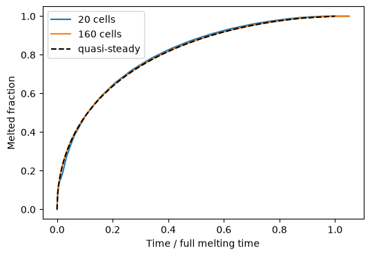
Both meshes follow the quasi-steady solution. Early on, a coarse mesh deviates slightly: the melting front crosses the large outer cells of the sphere one at a time (the enthalpy method with a sharp melting point). Refined, the model is within 1 % of the quasi-steady solution from half melted onwards.