Plot colours

PyTES has its own plot colours (DESIGN D15), chosen to stay readable with colour-vision deficiency and led by the brand orange:

• the colour cycles PyTES Thermal, for light backgrounds, and PyTES Thermal (dark), for dark ones, as the matplotlib styles "pytes.thermal" and "pytes.thermal_dark";

• the colourmaps ember (sequential) and thaw (diverging), perceptually uniform, registered with matplotlib as "pytes.ember" and "pytes.thaw" (and reversed, ending in _r) when pytes.plotting is imported.

They are available but not yet the default: matplotlib’s own colours apply until you ask for these. This notebook shows each of them on a packed bed charge.

Tutorial 5 introduces plotting PyTES solutions.

import matplotlib.pyplot as plt
import numpy as np
import pybamm
from matplotlib.colors import CenteredNorm

import pytes
from pytes import plotting

model = pytes.PackedBedModel()
solution = pybamm.Simulation(model).solve([0, 1800])

Colour cycles

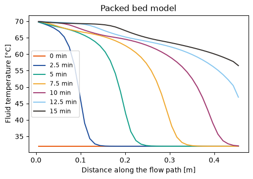
Use a cycle for one figure with plt.style.context, or for every figure with plt.style.use("pytes.thermal"). Seven fluid temperature profiles, every 2.5 minutes as the charge front crosses the bed, use all seven colours in order:

times = np.linspace(0, 900, 7)
with plt.style.context("pytes.thermal"):
    plotting.plot_fluid_profiles(solution, times)
    plt.show()

For dark backgrounds, combine a dark style with PyTES Thermal (dark), which comes second so that its colours win:

with plt.style.context(["dark_background", "pytes.thermal_dark"]):
    plotting.plot_fluid_profiles(solution, times)
    plt.show()

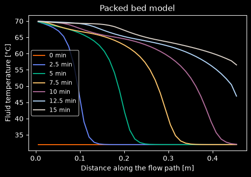
The colours are also plotting.THERMAL and plotting.THERMAL_DARK. A style does not reach pybamm.QuickPlot (and so Simulation.plot) until PyBaMM uses matplotlib’s colour cycle there (pybamm-team/PyBaMM#5953); meanwhile, pass the colours to it: pybamm.QuickPlot(solution, colors=list(plotting.THERMAL)).

Colourmaps

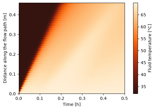
Ember runs from dark brown through the brand orange to cream, with lightness rising steadily and equal perceptual steps, so it suits a field such as the fluid temperature along the bed over time:

fluid = solution["Heat transfer fluid temperature [degC]"]
z = fluid.mesh.nodes
t = solution["Time [h]"].entries
T = fluid(t=solution.t, z=z)

fig, ax = plt.subplots(figsize=(5, 3.5), layout="constrained")
field = ax.pcolormesh(t, z, T, cmap="pytes.ember", shading="nearest")
fig.colorbar(field, label="Fluid temperature [°C]")
ax.set_xlabel("Time [h]")
ax.set_ylabel("Distance along the flow path [m]")
plt.show()

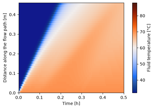
Thaw is diverging, from blue through a pale centre to orange. Centre it on a reference value with matplotlib’s CenteredNorm, here the PCM melting temperature: the pale band is the fluid at the melting temperature, orange above it and blue below. CenteredNorm makes the range symmetric about the centre, so a kelvin is the same step in colour on both sides, and the orange side stops short of its darkest red because the fluid never gets 28 K above the melting temperature. (TwoSlopeNorm would stretch each half over its own range, here 28 K below the centre and 10 K above, so that a kelvin would look 2.8 times bigger above it. It suits two sides that are not comparable, such as different units.)

T_melt = model.default_parameter_values["PCM melting temperature [K]"] - 273.15
norm = CenteredNorm(vcenter=T_melt)

fig, ax = plt.subplots(figsize=(5, 3.5), layout="constrained")
field = ax.pcolormesh(t, z, T, cmap="pytes.thaw", norm=norm, shading="nearest")
fig.colorbar(field, label="Fluid temperature [°C]")
ax.set_xlabel("Time [h]")
ax.set_ylabel("Distance along the flow path [m]")
plt.show()