Flow-dependent heat transfer coefficients

By default the heat transfer coefficient between the fluid and the storage is a constant parameter, "Heat transfer coefficient [W.m-2.K-1]". In practice it depends on the flow, so a value chosen at one flow rate does not hold at another. The option "heat transfer coefficient" computes it instead from a Nusselt number correlation, with the fluid properties from the fluid-property object and the geometry from the family:

• "Gnielinski" in the finned-tube models, for the flow inside the tubes;

• "Wakao-Kaguei" in the packed bed, for the flow around the capsules.

Every model outputs "Heat transfer coefficient [W.m-2.K-1]"; with a correlation it also outputs the surface Reynolds, Prandtl and Nusselt numbers.

import matplotlib.pyplot as plt
import numpy as np
import pybamm

import pytes

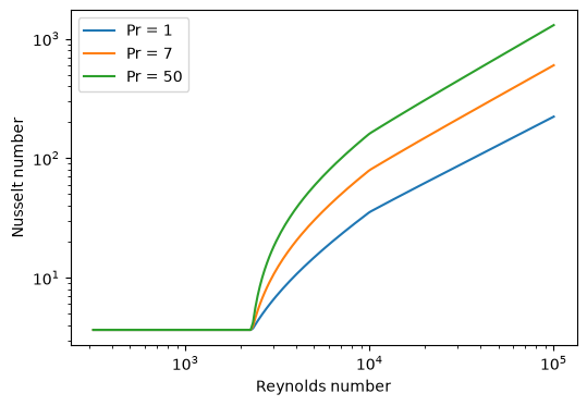
The Gnielinski law uses the laminar Nusselt number of a tube at a uniform wall temperature, 3.66, below a Reynolds number of 2300, the Gnielinski correlation above \(10^4\), and a linear interpolation in between.

Re = np.logspace(2.5, 5, 200)
fig, ax = plt.subplots(figsize=(6, 4))
for Pr in (1, 7, 50):
    Nu = pytes.submodels.Gnielinski(1).nusselt(pybamm.Vector(Re), pybamm.Scalar(Pr))
    ax.loglog(Re, Nu.evaluate(), label=f"Pr = {Pr}")
ax.set_xlabel("Reynolds number")
ax.set_ylabel("Nusselt number")
ax.legend()
plt.show()

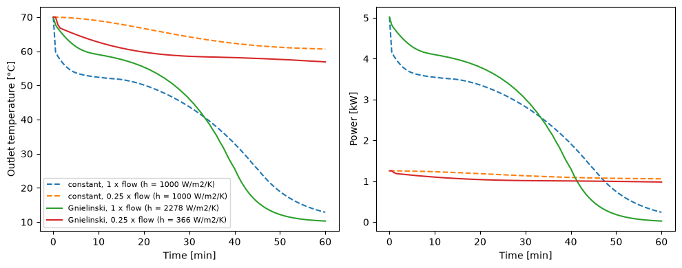
The default finned-tube battery runs at a Reynolds number of about 4200, in the transition, where the correlation gives a coefficient about twice the default constant. Here the battery is discharged at the default flow rate and at a quarter of it, which is laminar.

t = np.linspace(0, 3600, 121)
fig, axes = plt.subplots(1, 2, figsize=(10, 4))
for option, style in [("constant", "--"), ("Gnielinski", "-")]:
    model = pytes.SharpFrontModel(options={"heat transfer coefficient": option})
    for factor in (1, 0.25):
        parameter_values = model.default_parameter_values
        parameter_values["Mass flow rate [kg.s-1]"] *= factor
        solution = pybamm.Simulation(model, parameter_values=parameter_values).solve(
            [0, t[-1]], t_interp=t
        )
        h = solution["Heat transfer coefficient [W.m-2.K-1]"].entries[0]
        label = f"{option}, {factor:g} x flow (h = {h:.0f} W/m2/K)"
        time = solution["Time [min]"].entries
        axes[0].plot(
            time, solution["Outlet temperature [degC]"].entries, style, label=label
        )
        axes[1].plot(time, solution["Power [kW]"].entries, style, label=label)
axes[0].set_ylabel("Outlet temperature [°C]")
axes[1].set_ylabel("Power [kW]")
for ax in axes:
    ax.set_xlabel("Time [min]")
axes[0].legend(fontsize=8)
plt.tight_layout()
plt.show()

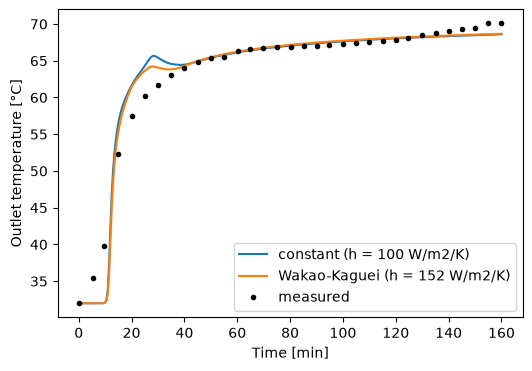
In the packed bed of Nallusamy et al. (2007), the Wakao and Kaguei correlation gives about 150 W.m-2.K-1, against the constant 100 of the default set, and fits the measured fluid temperature slightly better.

t_end = 160 * 60
t = np.linspace(0, t_end, 321)
t_data, T_data = np.loadtxt(
    "data/Nallusamy2007_HTF_1L.csv", delimiter=",", skiprows=1, unpack=True
)
fig, ax = plt.subplots(figsize=(6, 4))
for option in ("constant", "Wakao-Kaguei"):
    model = pytes.PackedBedModel(options={"heat transfer coefficient": option})
    solution = pybamm.Simulation(model).solve([0, t_end], t_interp=t)
    h = solution["Heat transfer coefficient [W.m-2.K-1]"].entries[0]
    ax.plot(
        solution["Time [min]"].entries,
        solution["Outlet temperature [degC]"].entries,
        label=f"{option} (h = {h:.0f} W/m2/K)",
    )
ax.plot(t_data, T_data, "ko", markersize=3, label="measured")
ax.set_xlabel("Time [min]")
ax.set_ylabel("Outlet temperature [°C]")
ax.legend()
plt.show()

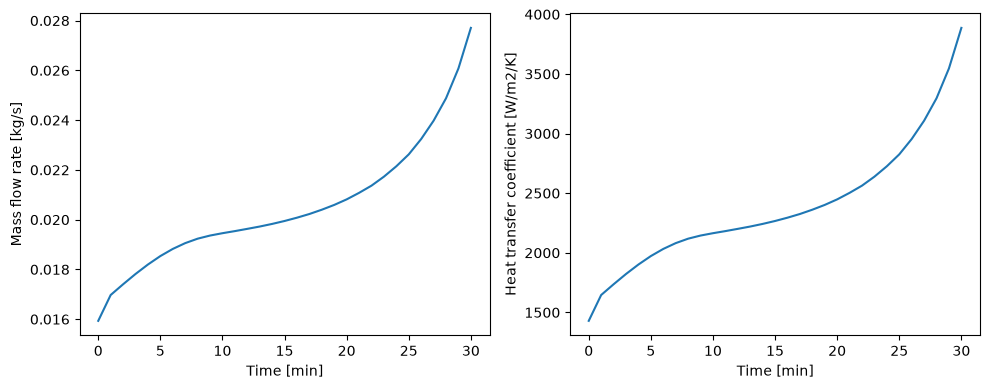
Under an experiment that adjusts the flow rate, such as a constant power discharge, the coefficient follows the flow.

model = pytes.SharpFrontModel(options={"heat transfer coefficient": "Gnielinski"})
experiment = pytes.experiments.Experiment(
    [pytes.experiments.step.Power(4000, inlet_temperature=283.15, duration=1800)]
)
solution = pytes.experiments.run_experiment(model, experiment)
fig, axes = plt.subplots(1, 2, figsize=(10, 4))
time = solution["Time [min]"].entries
axes[0].plot(time, solution["Mass flow rate [kg.s-1]"].entries)
axes[0].set_ylabel("Mass flow rate [kg/s]")
axes[1].plot(time, solution["Heat transfer coefficient [W.m-2.K-1]"].entries)
axes[1].set_ylabel("Heat transfer coefficient [W/m2/K]")
for ax in axes:
    ax.set_xlabel("Time [min]")
plt.tight_layout()
plt.show()

A correlation of your own

A correlation is only its Nusselt number: the family supplies the geometry (here the tube diameter, and the mean velocity in a tube) and the fluid-property object the properties. register_correlation adds a function of the Reynolds and Prandtl numbers, as PyBaMM symbols, as a value of the option for the models of its flow geometry, "tube" or "packed bed". PyTES adds its own correlations the same way. replace=True lets the cell run again.

Here the Dittus-Boelter correlation, for a fluid being heated, is compared with Gnielinski at four times the default flow, where both apply (\(Re > 10^4\)). conformance.check_model (in pytes.conformance) runs the contract on the model, energy conservation included, and returns its solution.

from pytes import conformance


def dittus_boelter(Re, Pr):
    return 0.023 * Re**0.8 * Pr**0.4


pytes.submodels.register_correlation(
    "Dittus-Boelter", dittus_boelter, flow="tube", replace=True
)
print(pytes.SharpFrontModel.allowed_options["heat transfer coefficient"])

for option in ("Gnielinski", "Dittus-Boelter"):
    model = pytes.SharpFrontModel(options={"heat transfer coefficient": option})
    parameter_values = model.default_parameter_values
    parameter_values["Mass flow rate [kg.s-1]"] *= 4
    solution = conformance.check_model(model, parameter_values)
    Re = solution["Surface Reynolds number"].entries[0]
    h = solution["Heat transfer coefficient [W.m-2.K-1]"].entries[0]
    print(f"{option}: Re = {Re:.0f}, h = {h:.0f} W/m2/K")

HeatTransferCoefficientOptions('tube'): ['constant', 'Gnielinski', 'Dittus-Boelter']

Gnielinski: Re = 16977, h = 12813 W/m2/K

Dittus-Boelter: Re = 16977, h = 12106 W/m2/K

A law that is not a Nusselt correlation, such as a wall resistance in series or a nonlinear law, goes to the coupling through the composition API instead (see composing models).